
How to Create a Sankey Chart in Excel Spreadsheet?
Insert the diagram. To insert a new diagram, select the data, and click the Sankey icon: After clicking the icon, the add-in generates the flow diagram in real time and shows the connections between stages. The diagram transforms the cash-flow data into a stunning visualization.
How to draw Sankey diagram in Excel? My Chart Guide
Step 3: Generate a Stacked Bar Chart. Excel doesn't have a native Sankey chart, but you can simulate it using a stacked bar chart. Here's how: Select your data table. Go to the "Insert.
The Data School How to create a Sankey chart.
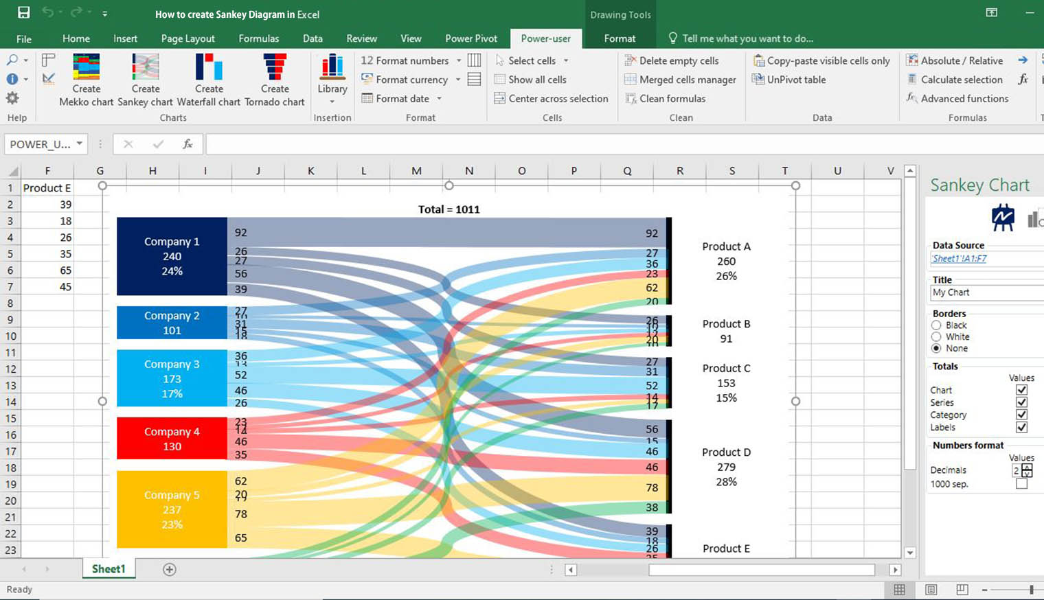
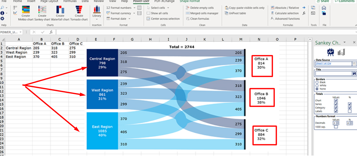
Creating a Sankey chart with Power-user. Currently, Sankey charts can only be created from the Excel ribbon of Power-user. From Excel, click Create Sankey chart. A dialog box will open, asking you to select the data source. Select your data, including the row and column headers, and click OK to validate. The chart will be created automatically.
How to Create Sankey Diagram in Excel? Easy Steps
Click Sankey Chart. Select the variables: Type, Main Source, and Source type, Energy Source, Usage, End User, Mega Watt . Click on Create Chart from sheet data, as shown below. Let's check out our resulting chart. You have the freedom to edit the chart to highlight key Just press the Edit Chart button, as shown above.
The Data School How to create a Sankey chart.
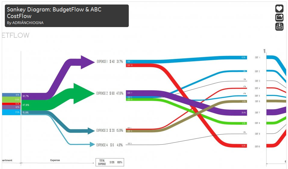
These chart types are available in Power BI, but are not natively available in Excel. However, today I want to show you that it is possible to create a Sankey diagram in Excel with the right mix of simple techniques. While Sankey diagrams are often used to show energy flow through a process, being a finance guy, I've decided to show cashflow.
How to Create a Sankey Diagram in Excel? eForbes
Gather your website visitors' data and analyze with Sankey Diagram in Excel and Google Sheets in a few clicks. You can create Sankey Chart with up to 8 level.

Sankey Diagrams Excel
Creating a Sankey Diagram in Excel is a complex task without using 3rd party add-ins like Ultimate Dashboard Tools. The add-in provides a user-friendly interface to create these diagrams without getting into the coding. Here are the steps to create a Sankey Diagram in Excel: Install UDT chart utility for Excel. Select data, then click the.

[DIAGRAM] Sankey Diagram D3 Excel
Now, you need to draw the Sankey pillars to complete the diagram. To do this, select the B28:C34 cells >> click on the Insert tab >> Insert Column or Bar Chart tool >> 100% Stacked Column option. As a result, a stacked chart will appear. Now, go to the Chart Design tab >> Change Chart Type tool.

[12+] Downloadable Sankey Diagram Excel And The Description [+] Z STUDENT
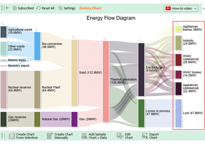
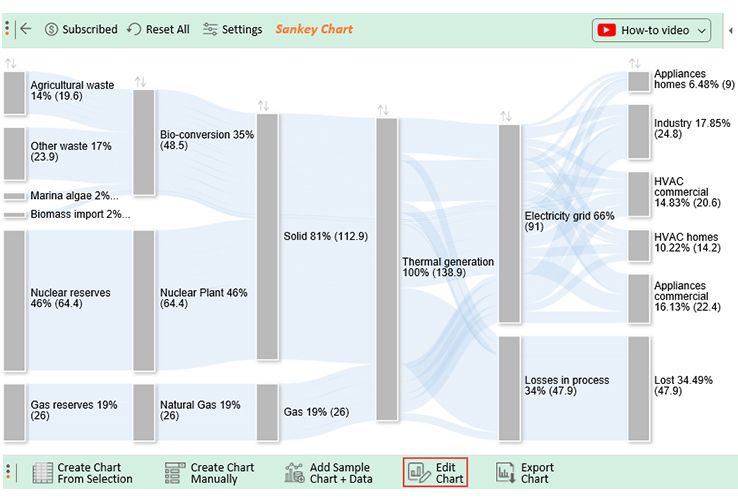
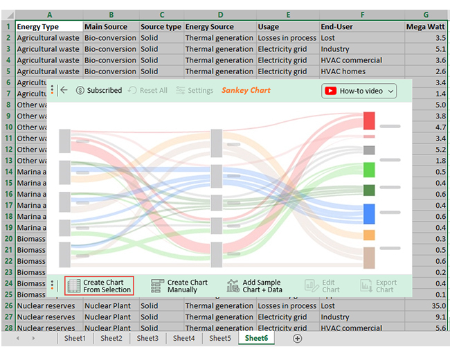
On your worksheet menu, click on Insert. The Insert menu will display the My Apps. Select ChartExpo add-in and click the Insert. Click on the " Sankey Chart " in the list of available charts in Excel, as shown below. After selecting the data click on Create Chart From Selection button, as shown below.
Sankey diagrams with Excel iPointsystems
A Sankey Diagram, or energy flow chart, is a type of data visualization that shows the path and quantity of data through various phases, categories or stages. While it started as a means to literally see how energy flows in an engineering system, the Sankey Diagram now has many applications and purposes.

Poweruser Create Sankey charts in Excel Poweruser
Open Excel and select the data you want to use for your Sankey diagram. Click on the Insert tab and select the SmartArt feature. From the SmartArt options, select the Flowchart category and choose the Basic Flowchart: Process option. Enter the node labels and link labels in the SmartArt diagram.
How to Create a Sankey Diagram in Excel? Easy to Follow Steps
★ Want to automate Excel? Check out our training academy ★ https://exceloffthegrid.com/academy★ Download the example file:★ https://exceloffthegrid.com/sanke.

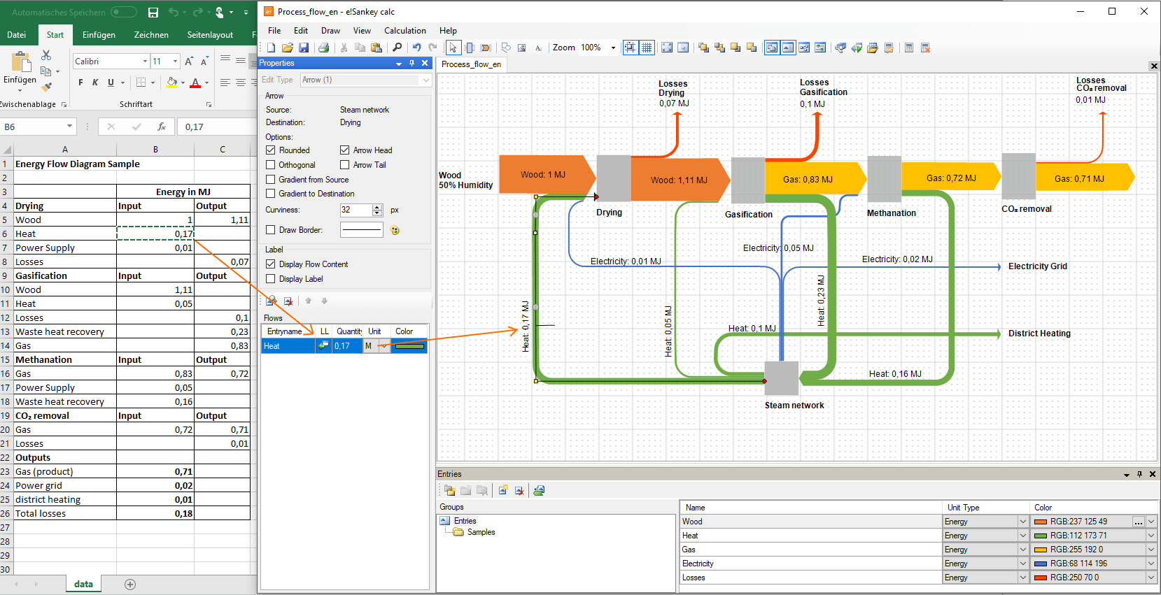
SankeyDiagramme erstellen mit e!Sankey show the flow
First, create a named range called "Blank" under the above table and give a suitable value. This value will be the width of the blank space inside the Sankey Chart. Next, you have to create the Sankey lines table. In this Sankey lines table, you have to insert all possible combinations of rows and columns wise.

How to create a Cash Flow Chart in Excel Sankey Diagram in Excel Cash Flow Chart YouTube
@Tom_By Here are two 3rd party add-ins that support Sankey Diagram: The first is a complex data visualization tool: Ultimate Dashboard Tools for Excel. Another great solution is the Power-user add-in. Both of them provide advanced charts and graphs for Excel.
Sankey Diagrams Excel
Let us take a look. Start by opening your MS Excel sheet and enter the data that you want to be transformed into a chart. On the top, on the tool bar, you will find the "Power User" tab. Click on that and you will find the Create Sankey Chart Option. Select the cells with the input data and then click on "OK" to proceed creating the chart.
How to Create Sankey Diagram in Excel? Easy Steps
b. Insert a Sankey chart: Select the data range, go to the Insert tab, and choose the Sankey chart option. Excel will generate a basic Sankey chart based on your data. c. Customize the chart: Format the chart by adjusting colors, line thickness, labels, and other visual elements to enhance clarity and aesthetics.